Documentation

1 Installation

1.1 Installing Galaxia

1.1.1 Installation

Note there are also instructions from the creators of Galaxia at http://galaxia.sourceforge.net/Galaxia3pub.html; what follows is a very explicit version of that.

1. Go to https://sourceforge.net/projects/galaxia/files/ and download Galaxia by clicking the big green button.

2. Go to your Downloads folder and untar the file by double-clicking it.

3. Move the untar’d folder (which should be called something like galaxia-0.7.2) to your home directory. (That’s the directory where you get sent if you cd and don’t put a location).

4. In your home directory, make a directory called GalaxiaData (i.e. mkdir GalaxiaData).

5. Move to the galaxia-0.7.2 directory (i.e. cd galaxia-0.7.2), and in there, do the following (replacing /your/home/directory/ with your home directory as appropriate):

   ./configure --datadir=/your/home/directory/GalaxiaData/
   make
   sudo make install
   cp -r GalaxiaData/ /your/home/directory/GalaxiaData/
   

6. Move back into your home directory (i.e. cd), then run the following:

   galaxia -s warp
   

That should be it! You don’t have to install ebf if you just download PopSyCLE!

NOTE: the instructions in step 5 are assuming a root install. If you want to do a local install, you need to have a folder for the software to be installed in. For example, in my home directory I made a sw directory (/your/home/directory/sw) for Galaxia to be installed in. You can then run the following instead:

./configure --prefix=/your/home/directory/sw --datadir=/your/home/directory/GalaxiaData/
make
make install
cp -r GalaxiaData/ /your/home/directory/GalaxiaData/

You also need to export Galaxia to your path. In your .bash_profile or .zshenv add the line export PATH=\$PATH:/your/home/directory/sw/bin. Then proceed with step 6 in the installation instructions.

1.1.2 Uninstallation

You need to remove the compiled galaxia code (you can find where it is by typing which galaxia in the terminal), the GalaxiaData directory, and you might as well remove the galaxia-0.7.2 directory also. When you do which galaxia nothing should be returned.

1.1.3 Parameter modification

Suppose you want to change the pattern speed in Galaxia. To do this, follow the installation instructions up to and including step 4. Then do the following:

1. Move to the galaxia-0.7.2/src directory.

2. Open the Population.h file with your favorite text editor.

3. Find the pattern speed (in this case by searching for 71.62) and replace with your desired value (in this case 40.00).

4. Save the change.

Now return to step 5 in the installation instruction and proceed as instructed.

1.2 Installing SPISEA

SPISEA can be installed by cloning the repository from https://github.com/astropy/SPISEA and following the instructions.

1.3 Installing BAGLE

BAGLE can be installed by cloning the repository from https://github.com/MovingUniverseLab/BAGLE_Microlensing and following the instructions.

1.4 Installing Python libraries

We recommend the Anaconda distribution. See requirements.txt for details.

2 Reading Files

PopSyCLE uses all sorts of different file formats. It can easily get confusing, so here is a short guide to the basics.

2.1 How to read HDF5 files

Within the HDF5 file are datasets that store the information. It is kind of like a dictionary in python– the dataset can be manipulated just like a numpy array.

First, go to the directory containing the HDF5 file you want to open. Next, start ipython. Then type the following:

import h5py
hf = h5py.File('filename.h5', 'r')

If you want to see the names of all the datasets in an HDF5 file, type the following:

list(hf.keys())

Suppose you want to work with the dataset named dname

To access the dataset, type:

dset = hf['dname']

To view the columns of the dset, you can type:

dset.dtype.names

To access a column in the database, you can use the column names listed below. i.e. for mass of all the objects in a dataset you can use:

dset_masses = hf['dname']['mass']

Note that only one person at a time can work on an open HDF5 file. Thus, at the end, you need to close the file:

hf.close()

2.2 How to read EBF files

The EBF file is basically a dictionary in python. The output of Galaxia is in the EBF format.

First, go to the directory containing the EBF file you want to open. Next, start ipython. Then type the following:

from popsycle import ebf
ef = ebf.read('filename.ebf', '/')

If you want to see the names of all the keys in the EBF file, type the following:

ef.keys()

Suppose you want to work with the key xkey . To access that part of the file, type:

x = ef['xkey']

Now x is just a numpy array and can manipulated as such

You can also access just that key from the beginning instead of loading in the entire ebf file by:

ef = ebf.read('filename.ebf', '/xkey')

2.3 How to read FITS table files

First, go to the directory containing the fits file you want to open. Next, start ipython, Then type the following:

from astropy.table import Table
tab = Table.read('table.fits')

To view the entire table, just type tab . The table works similar to a python dictionary or like a pandas dataframe. The column names are the keys of the dictionary, and the dictionary name in this case is tab .

To view the header information/metadata, type

tab.meta

To view the column names type

tab.columns

3 Description of Pipeline

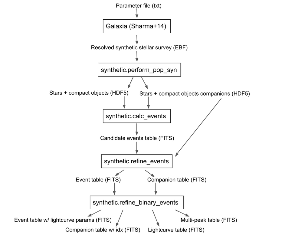
3.1 Pipeline without multiple systems

To run without companions, first, run Galaxia to create an EBF file, which produces a synthetic survey, i.e. a bunch of stars. Next, run population synthesis (perform_pop_syn) to inject compact objects into the synthetic survey; both the compact objects and stars are saved in an HDF5 file. Then run a synthetic survey (calc_events and refine_events) that will produce a list of microlensing events, which are listed in a FITS file.

3.2 Pipeline with multiple systems

To run with companions (with changed steps marked in bold), first, run Galaxia to create an EBF file, which produces a synthetic survey, i.e. a bunch of stars. Next, run population synthesis (perform_pop_syn) to inject compact objects and companions into the synthetic survey. Both the compact objects and stars are saved in an HDF5 file and the companions are stored in a separate hdf5 file. Then run a synthetic survey (calc_events and refine_events) that will produce a list of microlensing events, which are listed in a FITS file with a separate FITS file for associated companions after refine_events. Then model the binary lens events (refine_binary_events) which will produce some additional characteristics from the lightcurves and a description of all the peaks, which are listed in two FITS files.

4 Outputs

In addition to the outputs described below, each function produces a text log file that lists the input parameters

4.1 perform_pop_syn

4.1.1 Label/summary file (Astropy FITS Table)

• file_name is the name of the dataset for the HDF5 file.

• long_start and long_end are the edges of the longitude bin.

• lat_start and lat_end are the edges of the latitude bin.

• objects is the number of objects in that latitude/longitude bin.

• N_stars, N_WD, N_NS, and N_BH are the number of stars, white dwarfs, neutron stars, and black holes, respectively, in that latitude/longitude bin. The sum of these should be equal to the total number of objects.

Total white dwarfs is equal to adding the numbers of WDs made from MIST and the IFMR. WDs from the MIST models have photometry (they’re bright), while WDs from the IFMR and are dark (roughly 30th magnitude and below, so we assign them a value of nan for their magnitude.)

4.1.2 Stars and Compact Objects (primaries) (HDF5)

The data output contained in the HDF5 datasets are a combination of outputs that come directly from Galaxia, and outputs we ourselves have calculated or defined.

Default name: root.h5

Tag name	Brief Description	Units
zams_mass	ZAMS mass	M⊙
mass	Current mass	M⊙
systemMass	Sum of mass of primary and companions (if existent)	M⊙
px	Heliocentric x position	kpc
py	Heliocentric y position	kpc
pz	Heliocentric z position	kpc
vx	Heliocentric x velocity	km/s
vy	Heliocentric y velocity	km/s
vz	Heliocentric z velocity	km/s
age	Age	log(age/yr)
popid	Population ID - integer indicating the population type ranging from 0 to 9 (see Additional Descriptions below)	N/A
exbv	Extinction E(B-V) at the location of star given by 3-D Schlegel extinction maps	mag
glat	Galactic latitude	deg
glon	Galactic longitude	deg
mbol	Bolometric magnitude	log(L/L⊙)
grav	Surface gravity	log(gravity)
teff	Effective temperature	Log(T/Kelvin)
feh	Metallicity	[Fe/H]
rad	Galactic radial distance	kpc
isMultiple	True if the system has companions, False if the system does not	N/A
N_companions	Number of companions	N/A
rem_id	Integer indicating the remnant object type (see Additional Descriptions below)	N/A
obj_id	Object ID– unique integer to identify star/compact object	N/A
ubv_J, H, K, U, I, B, V, R	UBV photometric system, J, H, K, U, I, B, V, R system absolute magnitude	mag
ztf_g, r, i (optional)	ztf photometric system g, r, i absoltue magnitude	mag
vr	Galactic radial velocity	km/s
mu_b	Galactic proper motion, b component	mas/yr
mu_lcosb	Galactic proper motion, l component	mas/yr

Note that the tag names can be used to access HDF5 files (see “How to read HDF5 files” above). For stars (which are generated by Galaxia), the following outputs are taken directly from Galaxia and just reformatted into the HDF5 format; parenthetical names correspond to the tag name from Galaxia, if different: zams_mass (smass), mass (mact), px, py, pz, vx, vy, vz, age, popid, ubv_k, ubv_i, ubv_u, ubv_b, ubv_v, ubv_r, ubv_j, ubv_h, exbv (exbv_schlegel), teff, grav, mbol (lum), feh. Note that the lum key from Galaxia is referred to as mbol in the Galaxia documentation.

For compact objects (which we generated with our population synthesis code, SPISEA), we must assign these values ourselves.

For both stars and compact objects, the following are things we have directly calculated or assigned ourselves: rem_id, rad, glat, glon, vr, mu_b, mu_lcosb, obj_id. (For reasons relating to managing RAM, we calculate rad, glat, and glon although they are an output given directly from Galaxia, and we could have just read in the value. However, it can be calculated directly from knowledge of px, py, and pz.)

4.1.3 Stars and Compact Objects Companions (HDF5)

The data output contained in the HDF5 datasets are a combination of outputs that come directly from SPISEA , and outputs we ourselves have calculated or defined.

Default name: root_companions.h5

Tag name	Brief Description	Units
system_idx	System index corresponding to the obj_idx of the primary	N/A
zams_mass	ZAMS mass	M⊙
Teff	Effective Temperature	K
L	Luminosity	W
logg	Surface gravity	cgs
isWR	Is star a Wolf-Rayet?	N/A
mass	Current mass	M⊙
phase	Evolution phase (equivalent to rem_id in primary table)	N/A
metallicity	Companion metallicity	[Fe/H]
m_ubv_U, B, V, I, R	System magnitude in filters from SPISEA system	mag
m_ukirt_H, K, J	System magnitude in filters from SPISEA system	mag
m_ztf_g, r, i	System magnitude in filters from SPISEA system	mag
log_a	Log of the system semimajor axis	log(AU)
e	Eccentricity	N/A
i	Inclination	deg
Omega	Longitude of ascending node	deg
omega	Argument of periapsis	deg
zams_mass_match_diff	Difference between mass of SPISEA primary and matched Galaxia primary	ΔM⊙
zams_mass_prim	ZAMS mass of original SPISEA priamry	M⊙
spisea_idx	System index in original SPISEA systems table	N/A

4.2 calc_events

4.2.1 Event candidates table (Astropy FITS table)

The event candidates table is very similar to the HDF5 file created in perform_pop_syn. (In fact, the top part is completely duplicated; it’s here for completeness.)

However, the main difference is that there is a LOT less of the output, so instead of writing it in arrays in an HDF5 file, we use an Astropy table.

Each row in this table is associated with a microlensing event, each of which has a lens-source pair

Default name: root_events.fits

Tag name	Brief Description	Units
zams_mass (_L, _S)	ZAMS mass	M⊙
mass (_L, _S)	Current mass	M⊙
systemMass (_L, _S)	Sum of mass of primary and companions (if existent)	M⊙
px (_L, _S)	Heliocentric x position	kpc
py (_L, _S)	Heliocentric y position	kpc
pz (_L, _S)	Heliocentric z position	kpc
vx (_L, _S)	Heliocentric x velocity	km/s
vy (_L, _S)	Heliocentric y velocity	km/s
vz (_L, _S)	Heliocentric z velocity	km/s
age (_L, _S)	Age	log(age/yr)
popid (_L, _S)	Population ID - integer indicating the population type ranging from 0 to 9	N/A
exbv (_L, _S)	Extinction E(B-V) at the location of star given by 3-D Schlegel extinction maps	mag
glat (_L, _S)	Galactic latitude	deg
glon (_L, _S)	Galactic longitude	deg
mbol (_L, _S)	Bolometric magnitude	log(L/L⊙)
grav (_L, _S)	Surface gravity	log(gravity)
teff (_L, _S)	Effective temperature	Log(T/Kelvin)
feh (_L, _S)	Metallicity	[Fe/H]
rad (_L, _S)	Galactic radial distance	kpc
isMultiple (_L, _S)	True if the system has companions, False if the system does not	N/A
N_companions (_L, _S)	Number of companions	N/A
rem_id (_L, _S)	Integer indicating the remnant object type (more details in tag description)	N/A
obj_id (_L, _S)	Object ID– unique integer to identify star/compact object	N/A
ubv_J, H, K, U, I, B, V, R (_L, _S)	UBV photometric system, J, H, K, U, I, B, V, R absolute magnitude	mag
ztf_g, r, i (_L, _S) (optional)	ztf photometric system g, r, i absoltue magnitude	mag
vr (_L, _S)	Galactic radial velocity	km/s
mu_b (_L, _S)	Galactic proper motion, b component	mas/yr
mu_lcosb (_L, _S)	Galactic proper motion, l component	mas/yr
theta_E	(Angular) Einstein radius	mas
mu_rel	Relative source-lens proper motion	mas/yr
u0	(Unitless) minimum source-lens separation, during the survey	dimensionless (normalized to θE)
t0	Time at which minimum source-lens separation occurs	days

Tag names ARE used for the Astropy table. You will see a lot of the tag names have a parenthetical after (_L, _S). That is to indicate there is one tag for the lens (L) and one for the source (S), since for a given event, you need to have both a lens and a source, and each of these things has a mass, a velocity, a position, etc. For example, zams_mass_L is the ZAMS mass of the lens, and age_S is the log(age/yr) of the source.

4.2.2 Blends table (Astropy FITS table)

For each candidate microlensing event, associated with it are blended stars, which we call neighbors. Given the blend radius chosen when running calc_events, the blend table saves all neighbor stars that fall within that distance from the lenses in the candidate events table. The blends table is again almost identical to the HDF5 output, but is has three additional items. For each neighbor star, it lists the object ID of the lens and source it is associated with, and the distance between itself and the lens. Note that there can be multiple neighbor stars associated with a single lens and source (microlensing event).

Default name: root_blends.fits

Tag name	Brief Description	Units
zams_mass_N	ZAMS mass	M⊙
mass_N	Current mass	M⊙
systemMass_N	Sum of mass of primary and companions (if existent)	M⊙
px_N	Heliocentric x position	kpc
py_N	Heliocentric y position	kpc
pz_N	Heliocentric z position	kpc
vx_N	Heliocentric x velocity	km/s
vy_N	Heliocentric y velocity	km/s
vz_N	Heliocentric z velocity	km/s
age_N	Age	log(age/yr)
popid_N	Population ID - integer indicating the population type ranging from 0 to 9	N/A
exbv_N	Extinction E(B-V) at the location of star given by 3-D Schlegel extinction maps	mag
glat_N	Galactic latitude	deg
glon_N	Galactic longitude	deg
mbol_N	Bolometric magnitude	log(L/L⊙)
grav_N	Surface gravity	log(gravity)
teff_N	Effective temperature	Log(T/Kelvin)
feh_N	Metallicity	[Fe/H]
rad_N	Galactic radial distance	kpc
isMultiple_N	True if the system has companions, False if the system does not	N/A
N_companions_N	Number of companions	N/A
rem_id_N	Integer indicating the remnant object type (more details in tag description)	N/A
obj_id_N	Object ID– unique integer to identify star/compact object	N/A
ubv_J, H, K, U, I, B, V, R_N	UBV photometric system, J, H, K, U, I, B, V, R absolute magnitude	mag
ztf_g, r, i_N (optional)	ztf photometric system g, r, i absoltue magnitude	mag
vr_N	Galactic radial velocity	km/s
mu_b_N	Galactic proper motion, b component	mas/yr
mu_lcosb_N	Galactic proper motion, l component	mas/yr
obj_id_L	Object ID of the lens	N/A
obj_id_S	Object ID of the source	N/A
sep_LN	Separation between lens and neighbor	arcsec

Note that there is no additional companions table associated with calc_events. In order to cross reference between the events and companions, refine_events must be run first

4.3 refine_events

4.3.1 Events table (Astropy FITS table)

The output here is very similar to the candidate events table. In fact, part of it is completely duplicated. All tags listed in the event candidates table are also part of the events table. However, the following columns are also appended. NOTE: the entries for u0 and t0 are overwritten; the values for u0 and t0 returned from calc_events is different from that returned in refine_events. Each refine_events file requires you to choose a filter and extinction law; in this table we suppose filter x is chosen.

Default name: root_refine_events_filter_reddeninglaw.fits

Tag Name	Brief Description	Units
u0	(Unitless) minimum source-lens separation, during the survey	dimensionless
t0	Time at which minimum source-lens separation occurs	days
delta_m_x	Bump amplitude (difference in baseline and maximum magnification magnitude) in x-band	mag
pi_rel	Relative parallax	mas
pi_E	Microlensing parallax	dimensionless
t_E	Einstein crossing time	days
ubv_x_app (_L, _S)	UBV photometric system, x-band apparent magnitude, with extinction	mag
ubv_x_LSN	Blended magnitude in x-band (Apparent magnitude of source + lens + neighbors → “baseline mag”)	mag
f_blend_x	Source flux fraction (unlensed source flux divided by baseline) in x-band	dimensionless
cent_glon_x_N	Galactic longitude l of neighbor stars’ centroid	deg
cent_glat_x_N	Galactic latitude l of neighbor stars’ centroid	deg
ubv_x_app_N	Apparent magnitude of neighbor stars, x-band apparent magnitude	mag
pps_seed	Seed used in perform_pop_syn	N/A
gal_seed	Seed used in run_galaxia	N/A

4.3.2 Companions table (Astropy FITS table)

This table is very similar to the companion HDF5 file created in perform_pop_syn. In fact, part of it is completely duplicated. There is some additional information to index between this table and the events table and additional binary properties below. There is also no mass_match_diff column. Each row in this table is a companion associated with an event. So, if a system is lensed twice, its companions will be duplicated in this table.

Default name: root_refine_events_filter_reddeninglaw_companions.fits

Tag name	Brief Description	Units
prim_type	Type of primary associated with companion: ‘S’ if source or ‘L’ if lens	N/A
q	Companion mass/primary mass	dimensionless
sep	Projected angular separation between companion and primary	mas
P	Period of companion	years
obj_id_L	Object ID of the lens	N/A
obj_id_S	Object ID of the source	N/A
alpha	Angle between binary axis and North	deg
phi_pi_E	Angle between North and relative proper motion between the source and the lens	deg
phi	Angle between the relative proper motion and the binary axis	deg

4.4 refine_binary_events

In this section we simulate lightcurves for all the binary events that contain a binary and store the parameters. In the case of triple

lenses/sources we simulate multiple lightcurves and choose the one with the largest amplitude. The following are the examples of systems we simulate:

• Binary lens and binary source:

  • Primary lens + companion lens + primary source + companion source

• Triple lens and single source:

  • Primary lens + companion lens 1 + source

  • Primary lens + companion lens 2 + source

• Triple lens and binary source:

  • Primary lens + companion lens 1 + primary source + companion source

  • Primary lens + companion lens 2 + primary source + companion source

• Triple lens and triple source

  • Primary lens + companion lens 1 + primary source + companion source 1

  • Primary lens + companion lens 1 + primary source + companion source 2

  • Primary lens + companion lens 2 + primary source + companion source 1

  • Primary lens + companion lens 2 + primary source + companion source 2

The parameters for all these lightcurves are stored in the lightcurves.fits table (see 4.4.5) where each bullet point would be an entry in that file. We then choose the lightcurve with the largest Δm as the microlensing event whose parameters are used in other tables. Whether it was used or not is indicated in the lightcurve.fits table.

4.4.1 Events table (Astropy FITS table)

This table is a duplicate version of the events table from refine_events with some additional properties below from the simulated lightcurves.

Default name: root_refine_events_filter_reddeninglaw_rb.fits

Tag name	Brief Description	Units
n_peaks	Number of peaks in lightcurve	N/A
bin_delta_m	Bump amplitude (difference in baseline and maximum magnification magnitude)	mag
tE_sys	Empirical Einstein crossing time (when the system magnitude is at least 10% the maximum magnitude)	days
tE_primary	Empirical Einstein crossing time of the peak of max mag (when the system magnitude is at least 50% the maximum magnitude of peak)	days
primary_t	Time at which maximum peak occurs	days
avg_t	Average time the peaks occur	days
std_t	Standard deviation of times peaks occur	days
asymmetry	Asymmetry as defined by Chebyshev Polynomials (see Additional Descriptions below)	dimensionless
companion_idx_list	List of companion indices associated with events (corresponds with companion_idx in the companions table)	N/A

4.4.2 Companions table (Astropy FITS table)

This table is a duplicate version of the companions table from refine_events with an additional id Default name: root_refine_events_filter_reddeninglaw_companions_rb.fits

Tag name	Brief Description	Units
companion_idx	Companion index which corresponds to position in the array	N/A

4.4.3 Multi-peak table (Astropy FITS table)

This table describes properties of each of the peaks in a binary lens microlensing event lightcurve that passed a significance threshold of 10-5 (by default).

Default name: root_refine_events_filter_reddeninglaw_companions_rb_mp.fits

Tag name	Brief Description	Units
comp_id	Companion ID - the position of associated companion in companion table	N/A
obj_id_L	Object ID of the lens	N/A
obj_id_S	Object ID of the source	N/A
n_peaks	Number of peaks in lightcurve	N/A
t	Time at which peak occurs	days
tE	Empirical Einstein crossing time of the peak (when the system magnitude is at least 50% the maximum magnitude of peak)	days
delta_m	Bump amplitude (difference in baseline and maximum magnification magnitude of peak)	mag
ratio	Magnitude ratio between peak of the maximum mag and this peak	dimensionless

4.4.4 Lightcurve table (Astropy FITS table)

This table has the parameters of all the lightcurves simulated. In any cases involving a binary lens or source but no triples, there will be only one lightcurve for that event. However, in triple lens or triple source cases there will be 2 lightcurves in the TSBL, TSPL, BSTL, and PSTL cases and 4 lightcurves in the TSTL case.

Tag name	Brief Description	Units
obj_id_L	Object ID of the lens	N/A
obj_id_S	Object ID of the source	N/A
companion_L	Companion ID of the lens (blank if BSPL)	N/A
companion_S	Companion ID of the source (blank if PSBL)	N/A
class	Type of microlensing event simulated (PSBL, BSPL, or BSBL)	N/A
n_peaks	Number of peaks in lightcurve	N/A
bin_delta_m	Bump amplitude (difference in baseline and maximum magnification magnitude)	mag
tE_sys	Empirical Einstein crossing time (when the system magnitude is at least 10% the maximum magnitude)	days
tE_primary	Empirical Einstein crossing time of the peak of max mag (when the system magnitude is at least 50% the maximum magnitude of peak)	days
primary_t	Time at which maximum peak occurs	days
avg_t	Average time the peaks occur	days
std_t	Standard deviation of times peaks occur	days
asymmetry	Asymmetry as defined by Chebyshev Polynomials (see Additional Descriptions below)	dimensionless
used_lightcurve	If this lightcurve had the largest bin_delta_m of the set, it will be used in the other tables corresponding to this event (True). If not, False.	N/A (bool)

4.5 Additional descriptions of tags

rem_id/phase: These label the different types of remnant objects (star, black hole, neutron star, or white dwarf). They are identified as following:

• 0: Star

• 101: White Dwarf

• 102: Neutron Star

• 103: Black Hole

pop_id: Describes which population is generated.

• 0: Thin disk, ≤0.15 Gyr

• 1: Thin disk, 0.15-1 Gyr

• 2: Thin disk, 1-2 Gyr

• 3: Thin disk, 2-3 Gyr

• 4: Thin disk, 3-5 Gyr

• 5: Thin disk, 5-7 Gyr

• 6: Thin disk, 7-10 Gyr

• 7: Thick disk, 11 Gyr (single-age)

• 8: Stellar halo, 14 Gyr (single-age)

• 9: Bulge, 10 Gyr (single-age)

• In Galaxia there is an option for a 10th population type; the Bullock and Johnston stellar halos. We have chosen not use it, and the code is not written to include it.

px, py, pz; vx, vy, vz: These are given in heliocentric coordinates (i.e. Cartesian coordinates with the sun at the origin.) See subsection on coordinate systems for more information.

rad, glat, glon; vr, mu_b, mu_lcosb: These are given in galactic coordinates (i.e. spherical coordinates with the sun at the origin.) See subsection on coordinate systems for more information.

ubv_U, B, V, R, I, J, H, K; exbv: Photometry information is given in absolute magnitude. For NSs and BHs, all these values are nan to indicate they are dark. Note that for dark primaries with luminous companions, these values will be the system luminosity.

t0: Note that you can have a negative day (this just means time before the “zero” time, which is defined as the state of the system that is generated by Galaxia and the population synthesis. Since we are assuming everything moves in straight lines, we can propagate either forward or backwards.) This can also be the case for primary_t and t in the output of refine_binary_events.

asymmetry: Asymmetry as defined by (Night et al. 2008) where the light curve is fit by a Chebyshev polynomial to the 50th degree (Khakpash et al. 2021) and \(k = \left(\sum T^2_{\rm odd} / \sum T^2_{\rm even} \right)\). Here the T’s are the coefficients of the Chebyshev polynomial. A light curve is symmetric when k = 0.

5 Coordinate Systems

There are two different coordinate systems used, Heliocentric and Galactic. Heliocentric coordinates are Cartesian coordinates with the sun at the origin. The positive \(x\) axis is pointing toward the Galactic Center, and the positive \(z\) axis is pointing toward the Galactic North Pole. Galactic coordinates are spherical coordinates with the sun at the origin. Longitude \(l\) is measuring the angular distance of an object eastward along the galactic equator from the galactic center, and latitude \(b\) is measuring the angle of an object north or south of the galactic equator (or midplane) as viewed from Earth; positive to the north, negative to the south. Radius \(r\) is the distance from the sun to the object.

The conversion between Heliocentric and Galactic is just the same as converting between rectangular to spherical coordinates, where \(\phi = l\) and \(\theta = -b + 90^{\circ}\). Going from Galactic to Heliocentric (units are degrees):

\(x = r\sin(-b + 90^{\circ}) \cos l = r \cos b \cos l\)

\(y = r\sin(-b + 90^{\circ}) \sin l = r \cos b \sin l\)

\(z = r\cos(-b + 90^{\circ}) = r\sin b\)

Going from Heliocentric to Galactic (units are degrees):

\(r = \sqrt{x^2 + y^2 + z^2}\)

\(b = -\cos^{-1}(z/r) + 90^{\circ}\)

\(l = \tan^{-1}(y/x)\)

Note: be careful with the branch of arctangent. Practically, use numpy.arctan2 if using Python.

Diagram of Heliocentric and Galactic coordinate systems. The red dot is the sun.